Generative AI 1.3: Probability and Statistics
In machine learning and generative AI, probability is used to model uncertainty and randomness, while statistics helps us make inferences about data. These concepts are foundational for understanding how models make predictions, how we can measure uncertainty, and how models like VAEs and GANs work.
1.3.1 Basic Concepts in Probability
Random Variables
A random variable is a variable that can take on different values according to some probability distribution. In machine learning, we often model data as random variables, because data can be noisy or incomplete.
- Discrete Random Variables: Take on a countable set of values (e.g., number of heads in coin tosses).
- Continuous Random Variables: Take on an uncountable range of values (e.g., height, temperature).
Example:
If \(X\) is a random variable representing the outcome of a coin flip:
- \(X = 1\) for heads,
- \(X = 0\) for tails.
Probability Distribution
A probability distribution describes how the probabilities are assigned to different values of a random variable. The distribution tells us how likely certain outcomes are.
Types of Distributions:
- Discrete Distribution (e.g., Bernoulli, Binomial):
- The Bernoulli Distribution models a binary random variable (e.g., a single coin flip with probability \(p\) of heads).
- Continuous Distribution (e.g., Normal/Gaussian, Uniform):
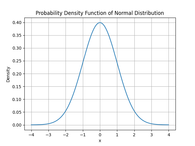
- The Normal Distribution (or Gaussian distribution) is one of the most common continuous distributions. It is defined by two parameters:
- \(\mu\) (mean): the center of the distribution,
- \(\sigma^2\) (variance): how spread out the distribution is.
- The Normal Distribution (or Gaussian distribution) is one of the most common continuous distributions. It is defined by two parameters:
1.3.2 Expectation, Variance, and Standard Deviation
Expectation (Mean):
The expectation or mean of a random variable is the average value it takes, weighted by its probabilities. It is denoted by \(\mathbb{E}[X]\).
Formula (Discrete Case):
\[\mathbb{E}[X] = \sum_x P(X = x) \cdot x\]Formula (Continuous Case):
\[\mathbb{E}[X] = \int_{-\infty}^{\infty} x \cdot P(X = x) dx\]Example:
For a fair coin flip (where \(P(X = 1) = 0.5\) and \(P(X = 0) = 0.5\)):
\[\mathbb{E}[X] = 1 \cdot 0.5 + 0 \cdot 0.5 = 0.5\]Variance and Standard Deviation
The variance measures how spread out the values of a random variable are. It is the expected value of the squared deviation from the mean. The standard deviation is simply the square root of the variance, providing a measure of spread in the same units as the data.
Variance Formula:
\[\text{Var}(X) = \mathbb{E}[(X - \mathbb{E}[X])^2]\]Standard Deviation:
\[\text{Std}(X) = \sqrt{\text{Var}(X)}\]1.3.3 Conditional Probability and Bayes’ Theorem
Conditional Probability
Conditional probability is the probability of an event occurring given that another event has already occurred. The conditional probability of event \(A\) given event \(B\) is denoted by \(P(A|B)\).
Formula:
\[P(A|B) = \frac{P(A \cap B)}{P(B)}\]Where:
- \(P(A \cap B)\) is the probability that both \(A\) and \(B\) occur,
- \(P(B)\) is the probability that \(B\) occurs.
Example:
If we know that 60% of students study math, and 30% of all students study both math and physics, then the probability that a student studies physics given that they study math is:
\[P(\text{Physics}|\text{Math}) = \frac{P(\text{Math} \cap \text{Physics})}{P(\text{Math})} = \frac{0.3}{0.6} = 0.5\]Bayes’ Theorem
Bayes’ Theorem relates conditional probabilities and allows us to update our beliefs based on new evidence. It is used in machine learning for probabilistic models like Naive Bayes and Bayesian Networks.
Formula:
\[P(A|B) = \frac{P(B|A) \cdot P(A)}{P(B)}\]Example:
Let \(A\) be the event “Student studies math,” and \(B\) be the event “Student passes the exam.” Bayes’ Theorem allows us to calculate \(P(A|B)\) (probability of studying math given that the student passed the exam) if we know the reverse probabilities.
1.3.4 Maximum Likelihood Estimation (MLE)
In machine learning, we often need to estimate the parameters of a probability distribution. Maximum Likelihood Estimation (MLE) is a method of finding the parameters that maximize the likelihood of the observed data.
Likelihood Function:
The likelihood is the probability of observing the data given the parameters \(\theta\) of the distribution. For a dataset \(D = \{x_1, x_2, \dots, x_n\}\), the likelihood is:
\[L(\theta) = P(D|\theta) = P(x_1|\theta) \cdot P(x_2|\theta) \cdot \dots \cdot P(x_n|\theta)\]In practice, we maximize the log-likelihood:
\[\log L(\theta) = \sum_{i=1}^n \log P(x_i|\theta)\]Example:
If we have a dataset of coin flips and want to estimate the probability \(p\) of getting heads, we use MLE to find the value of \(p\) that maximizes the likelihood of observing the given coin flips.
Using Probability and Statistics in Python
Let’s implement some of the core probability and statistics concepts in Python using NumPy.
Install scipy and matplotlib:
pip install scipy matplotlib
Python Code:
import numpy as np
from scipy.stats import norm

# 1. Generate data from a normal distribution
mean = 0
std_dev = 1
data = np.random.normal(mean, std_dev, 1000)

# 2. Calculate the mean, variance, and standard deviation
calculated_mean = np.mean(data)
calculated_variance = np.var(data)
calculated_std_dev = np.std(data)

print(f"Mean: {calculated_mean}")
print(f"Variance: {calculated_variance}")
print(f"Standard Deviation: {calculated_std_dev}")

# 3. Plot the probability density function of the normal distribution
import matplotlib.pyplot as plt

# Generate values for plotting
x_values = np.linspace(-4, 4, 1000)
y_values = norm.pdf(x_values, mean, std_dev)

plt.plot(x_values, y_values)
plt.title("Probability Density Function of Normal Distribution")
plt.xlabel("x")
plt.ylabel("Density")
plt.grid(True)
plt.show()
Output:
Mean: 0.01526403164834703
Variance: 1.0155684817884316
Standard Deviation: 1.007754392326042

Summary of Probability and Statistics Concepts:
- Random Variables are used to model uncertainty in machine learning. They can be discrete or continuous.
- Probability Distributions describe how the values of random variables are distributed.
- Expectation (Mean) is the average value a random variable takes, while variance measures the spread of the values.
- Conditional Probability tells us the probability of one event occurring given that another has occurred.
- Bayes’ Theorem relates conditional probabilities and allows us to update beliefs based on evidence.
- Maximum Likelihood Estimation (MLE) helps us estimate the parameters of a probability distribution that best explain the observed data.
Comments